AI Applications for Medical Accelerators

Accelerator Side

CAS Topical Course on Medical Accelerators · Jurmala, Latvia · June 2026

Dr. Adnan Ghribi — GANIL / CNRS-IN2P3 · adnan.ghribi@ganil.fr

Welcome. This lecture covers AI applied to the machine — the accelerator — not the patient. 3 use cases with live notebooks, 10 min of context first. Q&A at the end.

Lecture outline

Part 1  —  Introduction

Context  ·  Brief history of AI  ·  AI through the physicist lens

Part 2  —  AI in accelerators

A 30 years dive  ·  Practical foundations Practical applications  ·  Future directions & opportunities

Summary  ·  References

aghribi/cas2026-ai-medical-accelerators AccML review: aghribi.github.io/acc-ml-living-review

Three companion notebooks — open on Colab now:

• 01_fault_detection — autoencoder on RF waveforms
• 02_beam_tuning — Bayesian optimisation with Cheetah
• 03_surrogate_model — MLP surrogate + ensemble UQ

Time plan — 50 min talk + 10 min Q&A. Hard-stop the talk at 50 to protect questions. Part 1 (0–10): intro & scope 0–2.5 · what AI is/isn’t 2.5–4 · history 4–7 · physicist lens 7–10. Part 2 (10–47.5): 30-years dive 10–13 · foundations 13–18 · UC1 18–27 · UC2 27–36 · UC3 36–43 · future directions 43–47.5. Summary 47.5–50 · Q&A 50–60.

Three live notebooks — the code on the slides is the code in those notebooks, all runnable on Colab right now, no installation. A glossary of acronyms is at the very end, just before the backup slides.

Disclaimer — scope & slide guide

click me to know more

In scope — accelerator side

• RF fault detection
• Beam tuning & daily startup
• Surrogate models for beam physics
• Digital twins

Out of scope today

• Treatment planning
• Patient-facing clinical AI
• Radiobiology · Regulatory certification

→ covered in the companion lecture “AI — the medical side”.

Slide elements you will encounter

① Code block — executable companion notebook

model.fit(X_train)
anomaly_scores = model.predict(X_test)

② Concept box — key physics or ML idea

CONCEPT

Langevin dynamics ≡ stochastic gradient descent

③ Article references — bottom of slide

Kaiser et al., PRAB 27 (2024) · Duris et al., PRL 124 (2020)

④ GitHub — slides, notebooks & living review

aghribi/cas2026-ai-medical-accelerators

⑤ Colab notebook — open in browser, zero install

▶ Open in Colab 01_fault_detection · 02_beam_tuning · 03_surrogate

A glossary of acronyms is at the end of the deck, before the backup slides.

Orientation slide — two minutes at most. Left: what’s in and out of scope. Right: the five visual elements students will see throughout the lecture. After this: Part 1 Introduction.

Part 1

Introduction

Context  ·  Brief history of AI  ·  AI through the physicist lens

0–10 min. Four beats: what AI is and isn’t (scope the field honestly); a compact history from the McCulloch-Pitts neuron (1943) to the 2024 Nobel Prize in Physics; then the physics–ML bridge (Hopfield as collective behaviour, statistical mechanics, Langevin dynamics). Keep it brisk — the applied payload is Part 2.

What AI is — and isn’t

Artificial Intelligence

symbolic logic · expert systems · search & planning

Machine Learning

classical ML (SVM · RF · kNN) · probabilistic models · ★ Bayesian opt. / GP

Neural networks · Deep learning

★ autoencoders · ★ MLP surrogates · CNN / Transformer · deep RL · generative (VAE · diffusion · LLM)

★ Our BO/GP tool lives in this ring — classical ML, not a neural network: “AI” ≠ “deep learning”.

Demystified today — with live code

• ★ Autoencoder — fault detection
• ★ Bayesian opt. / GP — beam tuning
• ★ MLP surrogate — fast beam physics

Not covered here: symbolic AI · LLMs & agents · generative models — touched only in future directions.

Key idea

Match the method to your data — how much you have, and whether it is labelled — not to the hype.

~1.5 min, and the scope-setting slide for the whole lecture. The nested rings are the standard containment view — AI contains machine learning, which contains neural networks and deep learning — but read them as a physicist: each ring is a broader hypothesis class. The point to make explicitly, because it is the common misconception: AI is much wider than deep learning. Symbolic AI, expert systems, and search dominated the field for decades; LLMs and agents are a current frontier we only touch in the futures section. What this lecture builds and demystifies, with runnable code, are the three starred methods — and crucially one of them, Bayesian optimisation with Gaussian processes, is classical probabilistic ML, not a neural network at all. So even our own three use cases span two rings, not one. Everything else on this map is real AI we are deliberately not covering today.

A Brief History of AI

From the first neuron to the Nobel Prize in Physics

~9 minutes on history. The arc is deliberate: 1943 first mathematical neuron → 2024 Nobel Prize in Physics. The goal is not completeness but to make one point land — this is an 80-year-old, physics-rooted field, and its two “winters” teach healthy scepticism about hype cycles. Keep it brisk; the payoff is the physicist-lens section after.

From neuron to Nobel Prize (1943–2024)

The yellow dot at 2024 is the Nobel Prize in Physics awarded to Hopfield and Hinton — formally recognising that the foundations of modern AI are physics.

Note the two “winters” (after 1969 and after the late 1980s) — periods when funding and interest collapsed because the field overpromised. The current period since AlexNet in 2012 has been the longest sustained growth in AI history.

McCulloch & Pitts — the first artificial neuron (1943)

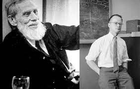
Warren McCulloch & Walter Pitts — first mathematical model of a neuron, mapping neural firing onto Boolean logic (1943).

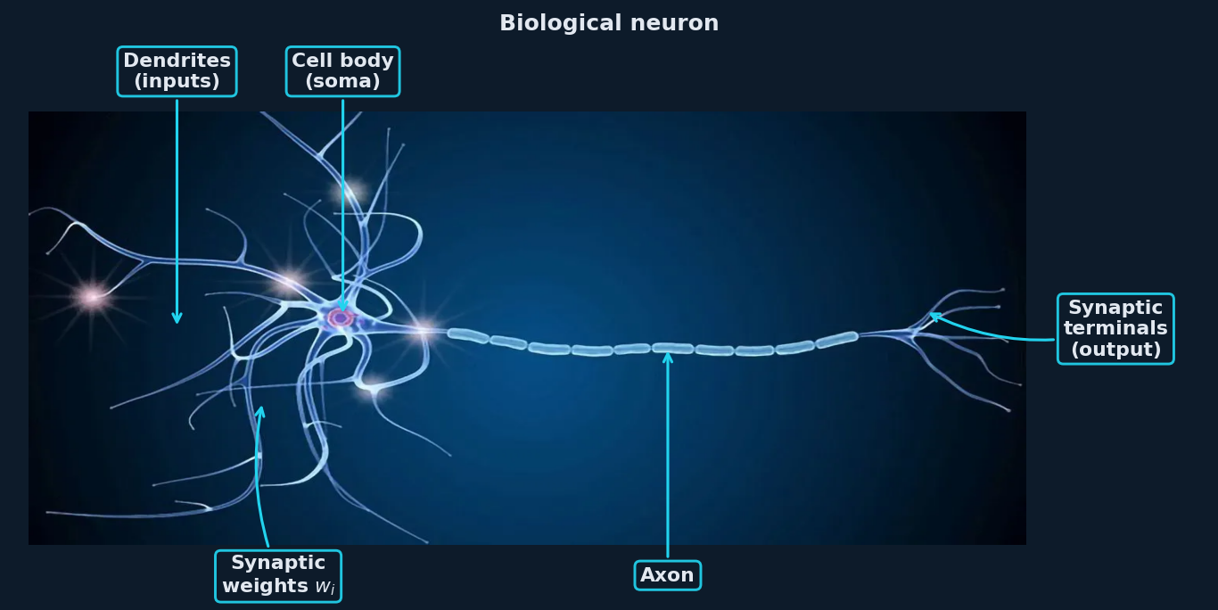
How a neuron works:

• Dendrites collect incoming signals from neighbouring neurons
• Soma integrates them as a weighted sum \(\sum w_i x_i\)
• Neuron fires if the sum exceeds threshold θ → signal propagates down the axon

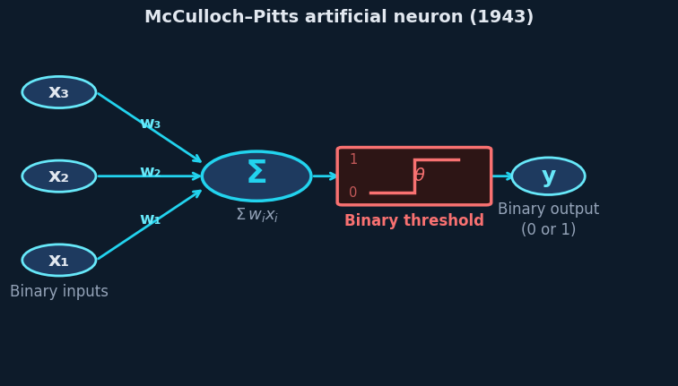
McCulloch & Pitts (1943). A logical calculus of the ideas immanent in nervous activity. Bull. Math. Biophysics 5, 115–133.

The starting point. McCulloch (a neurophysiologist) and Pitts (a logician) showed a neuron can be modelled as a threshold logic gate: take a weighted sum of inputs and fire if it exceeds a threshold θ. Two things to stress. First, the biological-to-mathematical mapping — dendrites are the inputs, the soma performs the weighted summation, the axon carries the output. Second, and crucially, the weights here are fixed by hand: there is no learning yet. Learning is what Rosenblatt adds on the next slide. So this is the architecture of a neuron without the ability to adapt.

The perceptron — first learning algorithm (1957)

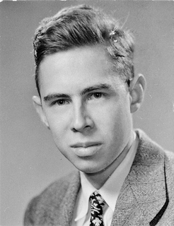
Frank Rosenblatt, 1957 — the Perceptron:

\[y = \text{sign}\!\left(\sum_i w_i x_i - \theta\right)\]

One neuron: \(N\) weighted inputs \(x_i\), one binary output \(y\). Unlike McCulloch-Pitts, the weights \(w_i\) are not fixed — they are learned from labelled examples via an error-correction rule.

The perceptron learning rule:

\[w_i \leftarrow w_i + \eta \cdot (y - \hat{y}) \cdot x_i\]

Every modern network still follows this principle.

Rosenblatt’s Mark 1 Perceptron (1958) was a physical hardware device — it made the front page of the New York Times.

Rosenblatt, F. (1958). The perceptron: a probabilistic model for information storage and organization in the brain. Psychol. Rev. 65(6), 386–408.

Is the perceptron “a single neuron”? Yes — exactly one neuron. The formula shows it: N inputs x_i each with a weight w_i, summed and passed through a sign function to give one binary output y. It is not a network; it is a threshold logic unit, just like McCulloch-Pitts. The key difference from M-P is what Rosenblatt added: the weights are not programmed by hand — they are adjusted automatically each time the neuron makes a mistake.

Relationship to Hebbian learning: Hebb (1949) proposed a biological rule — “neurons that fire together wire together”: w_ij increases when neurons i and j are simultaneously active. Rosenblatt was conceptually inspired by this, but his update rule fires on ERROR, not on co-activation. Formally: Δw_i = η·(y − ŷ)·x_i. If the output is correct (y = ŷ), nothing changes. Only a mismatch drives an update. This is error-correction, not Hebbian.

Distinction from backpropagation (1986): The perceptron uses a sign (step) activation — non-differentiable, so no gradient can propagate. Backprop requires smooth, differentiable activations (sigmoid, ReLU). The perceptron also has no hidden layers. Modern deep networks are descendants conceptually but not mathematically.

The Mark 1 Perceptron at Cornell learned to recognise letters from photographs. New York Times (1958): “New Navy Device Learns By Doing.” It was a physical machine wired with potentiometers as weights.

AI winters and the deep learning renaissance

click me to know more

1969 — First winter Minsky & Papert prove perceptron cannot solve XOR.

1986 — Backpropagation Gradients through layers — the key mathematical unlock.

2012 — AlexNet cuts ImageNet error by 10 pp. Same idea, scaled. Deep learning era begins.

The Minsky-Papert result was a setback — XOR requires a hidden layer, which the perceptron lacked. The real fix was the sigmoid: a smooth, differentiable activation that lets gradients flow backward through multiple layers. A step function has zero gradient almost everywhere. Backprop was actually derived by Werbos in 1974 but ignored; Rumelhart, Hinton & Williams popularised it in 1986. The second winter was driven by SVMs and kernel methods outperforming neural nets on small datasets. AlexNet won on GPUs — the compute unlock, not a conceptual breakthrough.

AI Through the Physicist Lens

Energy, spins, and statistical mechanics

Hopfield networks · Boltzmann machines · the physics–ML bridge

~8–12 min. Hopfield networks as spin glass systems, the Ising connection, statistical mechanics of learning, SGD as Langevin dynamics. The point: accelerator physicists are not outsiders in ML — the toolkit is the same. Keep brisk.

Physics at the core of AI

J. Hopfield

G. Hinton

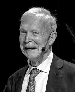
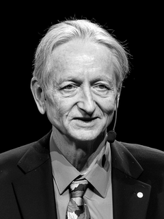
John Hopfield, 1982 — stores memories as energy minima of the Ising Hamiltonian:

\[E = -\frac{1}{2} \sum_{ij} w_{ij} s_i s_j\]

Geoffrey Hinton extended this with the Boltzmann distribution \(P(s) \propto e^{-E/T}\) — giving neural networks a thermodynamic learning rule.

Nobel Prize in Physics 2024

“for foundational discoveries enabling machine learning with artificial neural networks”

— John J. Hopfield & Geoffrey E. Hinton

Awarded in Physics, not Computer Science.

The Nobel Committee’s citation is explicit: Hopfield’s use of statistical mechanics to build associative memory, and Hinton’s extension to probabilistic models using the Boltzmann distribution, are the foundations.

As accelerator physicists, we think in terms of Hamiltonians, phase spaces, and energy minimisation every day. ML is a natural extension of our toolkit.

Hopfield networks — neurons as spins

click me to know more

A collective-effects view: a beam’s coherent modes emerge from pairwise particle interactions; a Hopfield memory emerges from pairwise neuron couplings. Both are many-body systems governed by an energy function.

The same mathematics describes Ising spins and neural networks:

Ising model	Hopfield network
Spin \(s_i \in \{-1,+1\}\)	Neuron state
Coupling \(J_{ij}\)	Synaptic weight \(w_{ij}\)
\(E = -\tfrac{1}{2}\sum J_{ij}s_is_j\)	Same Hamiltonian
Ground state	Stored memory

Red = −1 (spin ↓) · Cyan = +1 (spin ↑)

Hebbian learning — to store pattern \(\xi^\mu\): \[w_{ij} = \frac{1}{N}\sum_\mu \xi_i^\mu \xi_j^\mu\]

Hopfield, J.J. (1982). Neural networks and physical systems with emergent collective computational abilities. PNAS 79, 2554–2558.

Lead with the collective-effects framing (this is the hook for our audience): as accelerator physicists we never reason about one particle — we reason about the collective behaviour of the whole beam, where coherent modes, instabilities, and space-charge effects emerge from the pairwise interactions between particles, and the whole thing is governed by a Hamiltonian. A Hopfield network is the same kind of object: many simple units (neurons/spins), pairwise couplings, and a global energy whose minima are the interesting states. The difference is only what the minima mean — for a magnet, an ordered phase; for the network, a stored memory. So this is not a borrowed metaphor; it is the same many-body bookkeeping we already do for beams, applied to computation.

The table — Ising model and Hopfield network side by side:

The Ising model (Lenz 1920, Ising 1925) was invented to describe ferromagnetism. Every iron atom carries a magnetic moment (a spin) that can point up (+1) or down (−1). Neighbouring atoms interact: when both spins are aligned the energy is lower, so the system tends towards alignment. The total energy is E = −½ Σ_{ij} J_{ij} s_i s_j. In equilibrium the system sits at the minimum-energy configuration — all spins aligned (ferromagnet).

Hopfield’s 1982 insight: re-read those variables as a neural network: - Spin s_i ∈ {−1,+1} → neuron i is silent (−1) or active (+1). - Coupling J_{ij} between atoms i and j → synaptic weight w_{ij} between neurons i and j. - Energy minimum of the magnet → a stored memory pattern.

This is not an analogy — it is the same equation. A Hopfield network IS a physical spin system. The mathematics of ferromagnetism already contained the mathematics of associative memory; Hopfield made that explicit.

The Hebbian weight matrix — w_{ij} = (1/N) Σ_μ ξ_i^μ ξ_j^μ:

To store P patterns ξ^1, ξ^2, …, ξ^P (each a binary vector of ±1), you set the weight between neurons i and j to the average of their products over all stored patterns. If neurons i and j tend to be in the same state (both +1 or both −1) across many patterns, their weight is large and positive — exactly Hebb’s rule. Each pattern contributes one rank-1 outer-product matrix to W; the total weight matrix is their sum (normalised by N).

The figure — two heatmaps: - Left: the letter “H” encoded as a 10×10 grid. Cyan pixels = +1 (spin ↑), red pixels = −1 (spin ↓). This is the stored memory ξ. - Right: the same pattern with 28% of pixels randomly flipped. This is a corrupted or partial input given to the network at retrieval time. Despite 28% noise, the network converges back to the clean “H”. That is content-addressable memory: query with a fragment, retrieve the whole.

Statistical mechanics → deep learning

Physics concept	ML analogue
Hamiltonian / energy \(H(s)\)	Loss function \(\mathcal{L}(\theta)\)
Partition function \(Z = \sum_s e^{-H/T}\)	Normalisation constant (softmax, VAE)
Temperature \(T\)	Learning rate / annealing schedule
Boltzmann distribution \(P \propto e^{-E/T}\)	Softmax output — Boltzmann machine
Phase transition	Grokking (sharp generalisation threshold)
Langevin dynamics \(\dot{x} = -\nabla E + \eta\)	Stochastic gradient descent (SGD)
Free energy \(F = -T\ln Z\)	ELBO / variational lower bound (VAE)

Not metaphors — the same mathematics, rediscovered independently. As accelerator physicists we already speak this language.

Spend ~10 s here — point, don’t read. One sentence: every column is a physics concept the audience already owns, re-labelled for ML — the cleanest being “SGD ≈ Langevin dynamics.” Then move on; come back to any row only if asked.

Reference detail for questions: the SGD–Langevin connection was formalised by Welling & Teh (2011). The Boltzmann machine (Ackley, Hinton & Sejnowski 1985) is a literal physical model. Phase transitions in learning (grokking) are an active topic since Power et al. (2022). The deeper Hopfield capacity/retrieval material is now in the backup section if a question goes there.

Part 2

AI in accelerators

A 30 years dive  ·  Practical foundations Practical applications  ·  Future directions & opportunities

12–57 min. The core of the lecture: (1) a 30-year milestone dive through ML at accelerators; (2) the six AI application categories and the ML pipeline; (3) three hands-on use cases with live Python notebooks; (4) digital twins; (5) open problems and outlook.

A 30 Years Dive in AI for Accelerators

From research curiosity to operational tool

Milestones · concrete results · living review

~3 minutes. The message: AI at accelerators is not new — the first neural-network control work was 1992–94. Then two largely dormant decades, limited by compute, before the field reignited around 2016. End on the KARA −30% energy result, because it is measured on a real ring, not a simulation — proof that this is operational, not just a research curiosity.

30 years of AI at accelerators

Year	Facility	Approach	Impact
1992–94	Ion source · storage rings	Adaptive NN control (Mead+92); NN orbit correction (Bozoki & Friedman 94)	First ML for accelerator control
2020	SLAC LCLS	Bayesian optimisation in production	setup hours → ~tens of evaluations
2020	JLab CEBAF	ML on SRF cavity waveforms	Cavity-fault classification
2024	DESY / KIT	Cheetah differentiable simulator	10³–10⁵× faster than tracking codes
2020–23	CERN · DESY	Reinforcement learning for control & tuning	Autonomous closed-loop control
2024	KIT KARA	Anomaly detection + energy management	−30% energy footprint on real ring

Edelen et al., IEEE TNS 63 (2016) · Duris et al., PRL 124 (2020) · Kaiser et al., PRAB 27 (2024) · Ghribi et al., EPN 56 (2025)

30 years from first NNs to production AI systems. The earliest applications are Mead et al. (1992, adaptive NN control of an ion source) and Bozoki & Friedman (1994, NN orbit correction in storage rings) — then two dormant decades limited by compute, before project funding revived the field around 2016 (Edelen+2016). By 2020, BO was in production at LCLS (Duris+2020), with ML-based model-independent stabilisation demonstrated at ALS (Leemann+2019, PRL 123:194801) and differentiable simulation via Cheetah (Kaiser+2024, PRAB). Reinforcement learning entered control with sample-efficient RL at CERN (Kain+2020, PRAB 23:124801) and online RL+BO tuning at DESY (Kaiser+2023). KARA result is not a simulation — measured on the real machine.

AI in accelerators — concrete results

Fault detection — production ML triage

Beam tuning — BO + RL, closed-loop

Simulation — differentiable, fast surrogates

Optimisation toolboxes — facility-agnostic

Tennant et al., PRAB 23 (2020) · Duris et al., PRL 124 (2020) · Kaiser et al., PRAB 27 (2024) · Ghribi et al., EPN 56 (2025) · Zhang et al., IPAC 2022 (Badger)

These are production results, not simulations. CEBAF (JLab) has run ML-based SRF cavity-fault classification in production since ~2019 (Tennant et al. 2020 is a supervised classifier study; the unsupervised autoencoder in the live-demo notebook is our own illustration, not the CEBAF system). LCLS BO is the Duris+2020 PRL paper — real shots. KARA is the Ghribi+2025 EPN result with measured ring energy reduction. Badger (SLAC) and Geoff are open-source optimisation plugin frameworks that let operators swap algorithms (BO, Nelder-Mead, RL) without rewriting beamline code; both are in active production use at multiple facilities.

This living review covers all ML applications in accelerator physics — updated continuously. It is the map of what has been done and what is open. Bookmark it.

Five ways AI helps accelerators today

• Fault detection — classify anomalous events before interlocks trigger

• Beam tuning & adaptive control — optimal settings in < 50 evaluations; online RL in the loop

• Surrogate models — replace slow tracking codes (10³–10⁵× speedup)

• Predictive maintenance — forecast failures before they occur

• Digital twins — live virtual model of the actual machine, continuously updated

This lecture covers the first three in depth with runnable code.

Practical Foundations

From raw signals to trained model

Data · Features · Method selection · Pipeline

~7 minutes. Before the use cases, the unglamorous but decisive part: data quality, feature engineering, method selection, and the deploy pipeline. The theme to repeat throughout: in operational accelerator ML the bottleneck is almost never the model — it is the data and the integration into the control system.

The ML pipeline — from data to inference

Raw Data

Waveforms · images
logs · set-points

→

Pre-process

Clean · sync
normalise · resample

→

Feature extract

FFT · Gaussian fit
statistics · domain

→

Train & validate

80/20 split
cross-val · AUC

→

Deploy & infer

Sub-ms response
monitoring · retrain

UC1 · Fault detection

IQ waveforms → autoencoder → anomaly score

UC2 · Beam tuning

Quad settings → Cheetah → BO → proposal

UC3 · Surrogate

5 000 Cheetah calls → MLP → ~600× speedup

Road-map — present the full pipeline, then step through the highlighted sections before diving into each topic.

The ML pipeline — from data to inference

Raw Data

Waveforms · images
logs · set-points

→

Pre-process

Clean · sync
normalise · resample

→

Feature extract

FFT · Gaussian fit
statistics · domain

→

Train & validate

80/20 split
cross-val · AUC

→

Deploy & infer

Sub-ms response
monitoring · retrain

UC1 · Fault detection

IQ waveforms → autoencoder → anomaly score

UC2 · Beam tuning

Quad settings → Cheetah → BO → proposal

UC3 · Surrogate

5 000 Cheetah calls → MLP → ~600× speedup

① Data quality & preprocessing

Data quality and preprocessing — cleaning, synchronising, and normalising raw accelerator signals. This is what the next slides cover.

Raw Data

Waveforms · images
logs · set-points

→

Pre-process

Clean · sync
normalise · resample

Pause here — let the two boxes land. Next press reveals the full data quality content.

Raw Data

Waveforms · images
logs · set-points

→

Pre-process

Clean · sync
normalise · resample

① Clean Remove corrupted pulses, stuck sensors, dropouts.

② Synchronise Align timestamps across RF, BPM, power supplies.

③ Normalise Scale to [−1, 1] — prevents one channel dominating.

④ Balance SRF faults < 0.1 % of pulses — naïve model learns to ignore them.

A model trained on bad data learns bad behaviour.
No algorithm compensates for this.

Four preprocessing steps, ordered by how often they are skipped and later regretted. Each press lights up its panel in the strip below. Clean — remove corrupted pulses, stuck sensors, dropouts (panel 1: grey raw with two red outliers, cyan de-spiked result). Synchronise — align timestamps across RF, BPMs, and power supplies, genuinely hard across subsystems with different clocks (panel 2: two channels, one lagged). Normalise to [−1, 1] — so one high-amplitude channel does not dominate the loss (panel 3: scaled between the dotted bounds). Balance — SRF faults are under 0.1% of pulses, so a naïve model reaches 99.9% “accuracy” by always predicting normal and detecting nothing (panel 4: the log-scale class bar makes the imbalance visceral). Punchline on the overlay: a model trained on bad data learns bad behaviour, and no algorithm downstream compensates for that.

Raw Data

Waveforms · images
logs · set-points

→

Pre-process

Clean · sync
normalise · resample

→

Feature extract

FFT · Gaussian fit
statistics · domain

→

Train & validate

80/20 split
cross-val · AUC

→

Deploy & infer

Sub-ms response
monitoring · retrain

UC1 · Fault detection

IQ waveforms → autoencoder → anomaly score

UC2 · Beam tuning

Quad settings → Cheetah → BO → proposal

UC3 · Surrogate

5 000 Cheetah calls → MLP → ~600× speedup

② Feature engineering

You are here — feature extraction. p1 and p2 animate back from the top-left into the pipeline row.

Feature extract

FFT · Gaussian fit
statistics · domain

p3 shrinks and flies to top-left. Everything else disappears. Next press reveals feature engineering content.

Feature extract

FFT · Gaussian fit
statistics · domain

this case: 256 IQ samples → 3 scalars · 99 % compression, fault information retained

The feature map depends on the data — RF waveform → FFT peaks · Q · phase drift  ·  beam image → Gaussian-fit σ, centroid, image moments  ·  bunch → 6-D phase-space stats (emittance, Twiss α/β)  ·  BPM stream → orbit harmonics

Good features = simpler models + better generalisation.
Domain knowledge beats brute force.

The whole point of feature engineering in one figure: for this case, 256 raw IQ samples collapse to three physically meaningful scalars — mean amplitude, phase drift, fill fraction — with no loss of the information that distinguishes faults (99% compression). The strip beneath makes the general point: the right feature map depends on the data — FFT peaks/Q/phase for an RF waveform, Gaussian-fit σ and image moments for a screen image, 6-D phase-space statistics (emittance, Twiss) for a bunch, orbit harmonics for a BPM stream. Good features mean smaller models, less data, better generalisation: domain knowledge beats brute force. Then flag the trade-off that sets up UC1: this is the classical route, whereas the autoencoder deliberately skips hand-crafted features and learns its own representation from the raw waveform. Neither is universally right — it depends on how much you trust your physics versus your data.

Raw Data

Waveforms · images
logs · set-points

→

Pre-process

Clean · sync
normalise · resample

→

Feature extract

FFT · Gaussian fit
statistics · domain

→

Train & validate

80/20 split
cross-val · AUC

→

Deploy & infer

Sub-ms response
monitoring · retrain

UC1 · Fault detection

IQ waveforms → autoencoder → anomaly score

UC2 · Beam tuning

Quad settings → Cheetah → BO → proposal

UC3 · Surrogate

5 000 Cheetah calls → MLP → ~600× speedup

③ Train & validate

Third stage — train and validate. p4 lights up in the pipeline; the next press shrinks it into the top-left corner before the detail slide.

Train & validate

80/20 split
cross-val · AUC

p4 flies to the top-left corner and everything else clears. Next press brings in the train-and-validate detail.

Train & validate

80/20 split
cross-val · AUC

The task decides what “validate” means — and which metric.

Anomaly detection · UC1 unsupervised autoencoder

Validate on held-out normal + unseen fault types

✓ ROC-AUC · PR-AUC · F1

✗ accuracy — 99.9 % normal hides everything

Surrogate regression · UC3 supervised MLP

Validate on inputs outside the training points

✓ R² · RMSE · residual / σ

✗ extrapolation past the training envelope

Optimisation · UC2 Bayesian optimisation

No train/test split — judge best-so-far vs budget, across seeds

✓ regret · convergence · reproducibility

✗ trusting one lucky run

Same word, three protocols.
Anomaly & surrogate split the data; optimisation measures regret over a budget — there is no test set.

Before any loss curve, fix the most common confusion: “validate” is not one thing. Three task types, three protocols. Anomaly detection (UC1) is unsupervised — you validate the autoencoder on held-out normal data and, critically, on fault types it never saw in training; the metrics are ROC-AUC, precision-recall, F1, never raw accuracy, which is meaningless at 99.9% normal. Surrogate regression (UC3) is supervised — you hold out input points and check R², RMSE, and residuals against the model’s own uncertainty; the real failure mode is extrapolation outside the training envelope. Optimisation (UC2) is different in kind — there is no test set at all; you judge a Bayesian-optimisation run by its regret, its convergence against the evaluation budget, and whether it reproduces across random seeds, not by any single lucky run. The takeaway box: same word, three protocols. The next slide drills into the split-and-overfitting story, which applies to the first two.

Train & validate

80/20 split
cross-val · AUC

Train / validate / test — and the overfitting trap (supervised tasks)

Train · 70 %

Val · 15 %

Test · 15 %

fit the weights

tune & early-stop

touch once — unbiased estimate

⚡  Definition — Epoch

One epoch = one complete forward + backward pass over every training sample.
Example: 10 000 pulses, batch 32 → 313 weight updates per epoch.
Training halts when validation loss stops improving — the dashed line marks that minimum (early stopping).

Validate on data the model has never seen — and on faults it has never seen.
Temporal splits matter more than random splits in accelerator data — and stratify to preserve the < 0.1 % fault rate.

The three-way split, in order of who touches it: train fits the weights (blue, keeps falling); validation tunes hyper-parameters and triggers early stopping (cyan, U-shaped); test is the amber star — touched exactly once, at the chosen model, for an unbiased estimate (every extra peek leaks it into your choices). The loss curve is the overfitting story: train loss keeps falling while validation loss bottoms out and then turns back up — that widening gap is the model memorising noise, and early stopping freezes it at the validation minimum, where we read the test point. Define “epoch” from the concept box if the audience is mixed. Two accelerator-specific cautions on the last overlay: prefer temporal splits over random ones — random splits leak information between time-correlated neighbouring pulses and flatter the model — and stratify so the sub-0.1% fault rate survives in every split. With only hundreds of labelled faults, 5-fold cross-validation on the training portion is the practical way to get a stable estimate.

Raw Data

Waveforms · images
logs · set-points

→

Pre-process

Clean · sync
normalise · resample

→

Feature extract

FFT · Gaussian fit
statistics · domain

→

Train & validate

80/20 split
cross-val · AUC

→

Deploy & infer

Sub-ms response
monitoring · retrain

UC1 · Fault detection

IQ waveforms → autoencoder → anomaly score

UC2 · Beam tuning

Quad settings → Cheetah → BO → proposal

UC3 · Surrogate

5 000 Cheetah calls → MLP → ~600× speedup

④ Deploy & infer

Fourth and final stage — deploy and infer. p5 lights up; the next press shrinks it before the detail slide.

Deploy & infer

Sub-ms response
monitoring · retrain

p5 flies to the corner; next press brings in the deployment detail.

Deploy & infer

Sub-ms response
monitoring · retrain

① Latency budget Set by the control loop, not the model: fast feedback may need sub-ms, daily tuning tolerates seconds.

② Export & serve Deterministic runtime (e.g. ONNX, TorchScript) embeddable in EPICS / TANGO / DOOCS — no Python in the loop.

③ Compress to hardware Pruning + quantisation (FP32→INT8) cut latency — at some accuracy cost; trade-off depends on CPU / GPU / FPGA.

④ Monitor & retrain Track output rate and input distributions; retrain when drift crosses a threshold.

A model in a notebook is not a deployed model.
Latency, reliability and drift monitoring are engineering problems.

This is where most accelerator-ML projects actually fail. Four constraints, none about the model’s accuracy. Latency budget — set by the control loop, not the model: a fast feedback loop may demand sub-millisecond inference, while daily tuning tolerates seconds, so match the model to the loop’s deadline (don’t quote a universal number). Export and serve — convert to a deterministic runtime; ONNX and TorchScript are two examples, embeddable in EPICS / TANGO / DOOCS with no Python interpreter in the loop. Compress to the hardware — pruning and quantisation (e.g. FP32→INT8) cut latency and memory at some accuracy cost, and the right trade-off depends on whether you deploy on CPU, GPU, or FPGA. Monitor and retrain — track output rate and input distributions, retrain when drift crosses a threshold. The log-scale chart is illustrative (the dashed line is an example deadline). Closing line: a model in a notebook is not a deployed model — latency, precision, reliability, and drift are engineering problems, not modelling ones.

Practical Applications

Three use cases · Three live notebooks

Use case 1 — RF fault detection  ·  Use case 2 — Beam tuning  ·  Use case 3 — Surrogate models

Three back-to-back use cases, each self-contained. Same structure: problem → method → result → notebook. Companion notebooks are open on Colab.

Use Case 1

RF Fault Detection

Autoencoders on cavity IQ waveforms · Notebook 01

~11 minutes for UC1. The problem: rare RF faults with no labels. The method: an autoencoder trained on normal pulses only, with the anomaly score being the reconstruction error. Notebook 01 is live on Colab. Set expectations honestly here — be explicit later that this autoencoder is our own illustration on synthetic data, not the CEBAF production system, which is a supervised classifier (Tennant 2020).

The problem: rare faults, no labels

① Problem · ② Method · ③ Results · ④ Notebook

click me to know more

Every RF pulse → one IQ waveform per cavity at ~1 kHz. Clinical machines are safe by design — faults are rare.

Supervised classifiers need thousands of labelled fault examples per class — unavailable in clinical operation.

Solution: train on normal pulses only. Anomaly score = reconstruction error.

~1 kHz
IQ samples per cavity per second
1M+ pulses/day in clinical operation

Four fault classes — superconducting cavity

Class	Signature
Normal	Clean trapezoid · Q ≈ 0
Quench	Sudden drop mid flat-top
Detuning	Off-resonance · large Q
Multipacting	Oscillations on flat-top

No fault labels
needed
Anomaly detection trains on normal only

Frame the constraint honestly. Each cavity produces roughly 1 kHz of IQ waveforms — over a million pulses a day — but a clinical machine is safe by design, so genuine faults are vanishingly rare. That kills supervised classification: you cannot collect thousands of labelled examples per fault class in clinical operation. The reframe is the key insight: do not try to classify faults, instead model what “normal” looks like and flag anything that deviates. The four fault classes in the table — quench, detuning, multipacting, plus normal — are what we synthesise in the notebook to test the detector. The detector itself never sees them during training; it only ever learns normal.

What the waveforms look like

① Problem · ② Method · ③ Results · ④ Notebook

Row 1 = I (in-phase), Row 2 = Q (quadrature). Normal: clean trapezoid, Q near zero. Detuning: strong Q. Quench: sharp drop. Multipacting: oscillations.

The autoencoder — architecture

① Problem · ② Method · ③ Results · ④ Notebook

click me to know more

class RFAutoencoder(nn.Module):
    def __init__(self, latent_dim=16):
        super().__init__()
        self.encoder = nn.Sequential(
            nn.Conv1d(2, 32, kernel_size=8, stride=4),
            nn.GELU(),
            nn.Conv1d(32, 64, kernel_size=4, stride=2),
            nn.GELU(),
            nn.Flatten(),
            nn.Linear(64 * 32, latent_dim),  # bottleneck
        )
        self.decoder = nn.Sequential(...)    # mirror

class RFAutoencoder(nn.Module):
    def __init__(self, latent_dim=16):
        super().__init__()
        self.encoder = nn.Sequential(
            nn.Conv1d(2, 32, kernel_size=8, stride=4),
            nn.GELU(),
            nn.Conv1d(32, 64, kernel_size=4, stride=2),
            nn.GELU(),
            nn.Flatten(),
            nn.Linear(64 * 32, latent_dim),  # bottleneck
        )
        self.decoder = nn.Sequential(...)    # mirror

class RFAutoencoder(nn.Module):
    def __init__(self, latent_dim=16):
        super().__init__()
        self.encoder = nn.Sequential(
            nn.Conv1d(2, 32, kernel_size=8, stride=4),
            nn.GELU(),
            nn.Conv1d(32, 64, kernel_size=4, stride=2),
            nn.GELU(),
            nn.Flatten(),
            nn.Linear(64 * 32, latent_dim),  # bottleneck
        )
        self.decoder = nn.Sequential(...)    # mirror

class RFAutoencoder(nn.Module):
    def __init__(self, latent_dim=16):
        super().__init__()
        self.encoder = nn.Sequential(
            nn.Conv1d(2, 32, kernel_size=8, stride=4),
            nn.GELU(),
            nn.Conv1d(32, 64, kernel_size=4, stride=2),
            nn.GELU(),
            nn.Flatten(),
            nn.Linear(64 * 32, latent_dim),  # bottleneck
        )
        self.decoder = nn.Sequential(...)    # mirror

class RFAutoencoder(nn.Module):
    def __init__(self, latent_dim=16):
        super().__init__()
        self.encoder = nn.Sequential(
            nn.Conv1d(2, 32, kernel_size=8, stride=4),
            nn.GELU(),
            nn.Conv1d(32, 64, kernel_size=4, stride=2),
            nn.GELU(),
            nn.Flatten(),
            nn.Linear(64 * 32, latent_dim),  # bottleneck
        )
        self.decoder = nn.Sequential(...)    # mirror

Input (batch, 2, 256) — I and Q as two channels

① Encoder · lines 4–11 — two Conv1d stages compress the (2, 256) waveform.

② 1D convolutions · lines 5, 7 — capture local features (rise, drop, oscillations) with few parameters.

③ Bottleneck · line 10 — the pulse is squeezed through 16 numbers; the net must learn what normal looks like.

④ Decoder · line 12 — mirrors the encoder, rebuilding (2, 256) from the 16-D code.

Anomaly score = reconstruction error · Normal → low · Faults → high

2×256

→

32 ch

→

64 ch

→

16

→

64 ch

→

32 ch

→

2×256

◀ encoder · compress bottleneck decoder · reconstruct ▶

Arrow-driven walk-through. Each right-arrow press highlights the matching code lines on the left and lights up the corresponding point on the right; earlier points stay visible but dimmed (half-faded), so the list accumulates. The funnel below stays up throughout as the anchor. ① Encoder — two Conv1d stages compress the 2×256 input. ② 1D convolutions slide along the time axis, capturing local structure (rise, drop, oscillations) with far fewer parameters than dense layers. ③ Bottleneck — the whole pulse is squeezed through 16 numbers, so the network can only store a compact model of normal; this dimension is the critical hyperparameter (too large and it reconstructs faults too, killing the signal). ④ Decoder mirrors the encoder. Final press: the punchline — anomaly score = reconstruction error, low for normal, high for faults.

Training and result

① Problem · ② Method · ③ Results · ④ Notebook

# Train on NORMAL pulses only
X_normal = X_train[y_train == 0]
for epoch in range(50):
    for (batch,) in loader:
        loss = ((batch - model(batch))**2).mean()
        optimizer.zero_grad()
        loss.backward()
        optimizer.step()

# Score every pulse at inference
with torch.no_grad():
    scores = ((X - model(X))**2).mean(dim=(1,2))
threshold = scores[normal_mask].quantile(0.95)

# Train on NORMAL pulses only
X_normal = X_train[y_train == 0]
for epoch in range(50):
    for (batch,) in loader:
        loss = ((batch - model(batch))**2).mean()
        optimizer.zero_grad()
        loss.backward()
        optimizer.step()

# Score every pulse at inference
with torch.no_grad():
    scores = ((X - model(X))**2).mean(dim=(1,2))
threshold = scores[normal_mask].quantile(0.95)

# Train on NORMAL pulses only
X_normal = X_train[y_train == 0]
for epoch in range(50):
    for (batch,) in loader:
        loss = ((batch - model(batch))**2).mean()
        optimizer.zero_grad()
        loss.backward()
        optimizer.step()

# Score every pulse at inference
with torch.no_grad():
    scores = ((X - model(X))**2).mean(dim=(1,2))
threshold = scores[normal_mask].quantile(0.95)

# Train on NORMAL pulses only
X_normal = X_train[y_train == 0]
for epoch in range(50):
    for (batch,) in loader:
        loss = ((batch - model(batch))**2).mean()
        optimizer.zero_grad()
        loss.backward()
        optimizer.step()

# Score every pulse at inference
with torch.no_grad():
    scores = ((X - model(X))**2).mean(dim=(1,2))
threshold = scores[normal_mask].quantile(0.95)

① Train on normal only · lines 1–2 — the model never sees a fault.

② Reconstruction loss · lines 3–8 — minimise the MSE between each pulse and its rebuild.

③ Unsupervised threshold · lines 10–13 — flag pulses above the 95th percentile of normal errors. No fault labels used.

1.000
ROC-AUC — on synthetic data

Concept — ROC-AUC

A detector needs a threshold — but which one? ROC-AUC sidesteps the choice.
Sweep every threshold; at each, plot true-positive rate (sensitivity) vs false-positive rate (1 − specificity). AUC = area under that curve.
0.5 → coin-flip   1.0 → perfect separation of normal vs fault.
Threshold-independent — the right metric when a sub-0.1 % fault rate makes any single fixed cut arbitrary.

Two code ideas to highlight. First, we train only on normal pulses — the y==0 selection — so the network never sees a fault. Second, we set the decision threshold at the 95th percentile of the normal reconstruction errors: a purely unsupervised choice that needs no faults at all. The histogram then shows the payoff — normal errors cluster low, fault errors spread high, with clean separation at the threshold. The headline is ROC-AUC = 1.000, but say “on this synthetic dataset” out loud: real machines are messier and this number will not survive contact with real data — that gap is part of the open-problems discussion later. Use the ROC-AUC concept box for mixed audiences: it is threshold-independent, which is exactly why it is the right metric when no single fixed threshold is meaningful across operating conditions.

Notebook 01 — live preview

① Problem · ② Method · ③ Results · ④ Notebook

▶ Open 01_fault_detection in Colab

Live notebook — runnable on Colab from a phone, zero install. If time allows, walk through one cell: generating a normal pulse, training the autoencoder, then scoring a fault and watching the reconstruction error jump. Do not get stuck here — it is a pointer for the audience to explore later, not a deep dive.

Use Case 2

Beam Tuning with Bayesian Optimisation

Cheetah · differentiable accelerator simulation · Notebook 02

~11 minutes for UC2. The problem: daily beam tuning is slow and largely manual. The method: Bayesian optimisation on a Cheetah simulation. The deeper pedagogical payload — and the thing to keep coming back to — is dimensional scaling: in 2D, BO barely beats a grid, but the gap explodes as you add tuning dimensions. Notebook 02 is live.

The daily startup problem

① Problem · ② Method · ③ Results · ④ Notebook

click me to know more

Every morning on a clinical machine:

1. Run QA checks (output, flatness, energy)
2. Tune magnets until beam is within spec
3. Hand off to clinical staff

Currently: 20–45 min of physicist time, largely manual.

\(n\) correctors × \(k\) quads → high-dimensional space that grows exponentially for grid search.

Bayesian Optimisation fits naturally:

• Works in 2–20 dimensions
• ~50 evaluations to a good solution
• Model-free — no simulator needed

Demonstrated in production at SLAC LCLS and across light sources, FELs, and linacs (Duris 2020; Roussel et al. 2024).

Concept — Bayesian prior

A prior P(f) encodes your belief before data — e.g. “the beam response is smooth in magnet space”.
Bayes’ theorem updates it: P(f | data) ∝ P(data | f) · P(f) — the result is the posterior.
BO uses the posterior to pick the next probe: explore where uncertain, exploit where promising.
Every measurement actively informs the next — no wasted machine evaluations.

Ground the problem in daily operations. Every morning: run QA checks (output, flatness, energy), tune the magnets until the beam is within spec, then hand off to clinical staff. Today that is 20–45 minutes of largely manual physicist time. With n correctors and k quadrupoles the search space grows exponentially, so a grid scan is hopeless. BO fits this naturally: it works in 2–20 dimensions, reaches a good solution in tens of evaluations, and is model-free, so it runs directly on the machine with no simulator. Use the Bayesian-prior concept box to give the core idea: encode a belief — “the beam response is smooth in magnet space” — then let Bayes update it with each measurement so every probe is chosen to be maximally informative.

Cheetah — PyTorch beam dynamics

① Problem · ② Method · ③ Results · ④ Notebook

import torch, cheetah

# Beam diverges after a 2 m upstream drift
upstream = cheetah.Segment([cheetah.Drift(length=torch.tensor(2.0))])
beam_in  = upstream.track(cheetah.ParameterBeam.from_twiss(
    energy=torch.tensor(1088.3e6),   # 150 MeV proton, eV
    beta_x=torch.tensor(0.3),
    emittance_x=torch.tensor(1e-6),
    species=cheetah.Species("proton"),
))

# Re-focusing doublet
segment = cheetah.Segment(elements=[
    cheetah.Drift(length=torch.tensor(0.1)),
    cheetah.Quadrupole(length=torch.tensor(0.3), name="Q1"),
    cheetah.Drift(length=torch.tensor(0.6)),
    cheetah.Quadrupole(length=torch.tensor(0.3), name="Q2"),
    cheetah.Drift(length=torch.tensor(0.3)),
    cheetah.Screen(name="monitor"),
])

beam_out = segment.track(beam_in)

import torch, cheetah

# Beam diverges after a 2 m upstream drift
upstream = cheetah.Segment([cheetah.Drift(length=torch.tensor(2.0))])
beam_in  = upstream.track(cheetah.ParameterBeam.from_twiss(
    energy=torch.tensor(1088.3e6),   # 150 MeV proton, eV
    beta_x=torch.tensor(0.3),
    emittance_x=torch.tensor(1e-6),
    species=cheetah.Species("proton"),
))

# Re-focusing doublet
segment = cheetah.Segment(elements=[
    cheetah.Drift(length=torch.tensor(0.1)),
    cheetah.Quadrupole(length=torch.tensor(0.3), name="Q1"),
    cheetah.Drift(length=torch.tensor(0.6)),
    cheetah.Quadrupole(length=torch.tensor(0.3), name="Q2"),
    cheetah.Drift(length=torch.tensor(0.3)),
    cheetah.Screen(name="monitor"),
])

beam_out = segment.track(beam_in)

import torch, cheetah

# Beam diverges after a 2 m upstream drift
upstream = cheetah.Segment([cheetah.Drift(length=torch.tensor(2.0))])
beam_in  = upstream.track(cheetah.ParameterBeam.from_twiss(
    energy=torch.tensor(1088.3e6),   # 150 MeV proton, eV
    beta_x=torch.tensor(0.3),
    emittance_x=torch.tensor(1e-6),
    species=cheetah.Species("proton"),
))

# Re-focusing doublet
segment = cheetah.Segment(elements=[
    cheetah.Drift(length=torch.tensor(0.1)),
    cheetah.Quadrupole(length=torch.tensor(0.3), name="Q1"),
    cheetah.Drift(length=torch.tensor(0.6)),
    cheetah.Quadrupole(length=torch.tensor(0.3), name="Q2"),
    cheetah.Drift(length=torch.tensor(0.3)),
    cheetah.Screen(name="monitor"),
])

beam_out = segment.track(beam_in)

import torch, cheetah

# Beam diverges after a 2 m upstream drift
upstream = cheetah.Segment([cheetah.Drift(length=torch.tensor(2.0))])
beam_in  = upstream.track(cheetah.ParameterBeam.from_twiss(
    energy=torch.tensor(1088.3e6),   # 150 MeV proton, eV
    beta_x=torch.tensor(0.3),
    emittance_x=torch.tensor(1e-6),
    species=cheetah.Species("proton"),
))

# Re-focusing doublet
segment = cheetah.Segment(elements=[
    cheetah.Drift(length=torch.tensor(0.1)),
    cheetah.Quadrupole(length=torch.tensor(0.3), name="Q1"),
    cheetah.Drift(length=torch.tensor(0.6)),
    cheetah.Quadrupole(length=torch.tensor(0.3), name="Q2"),
    cheetah.Drift(length=torch.tensor(0.3)),
    cheetah.Screen(name="monitor"),
])

beam_out = segment.track(beam_in)

① Beam setup · lines 3–10 — a 150 MeV proton beam; after a 2 m drift it has diverged.

② Re-focusing doublet · lines 12–21 — two independently powered quads (Q1, Q2) and a screen.

③ Track · line 22 — push the beam through; read σ at the screen.

Why Cheetah? PyTorch module → gradients flow through the simulation · ms per call · same API for a virtual or real machine.

At the screen, quads off: σ_x + σ_y = 13.2 mm (6.6 mm/plane) — the baseline BO must beat.

 ·  Kaiser, Xu, Eichler & Santamaria Garcia, PRAB 27, 054601 (2024)

Cheetah is the enabling tool: a beam-dynamics code written as a PyTorch module. Two properties matter. It is differentiable — gradients flow straight through the tracking, so it composes natively with machine-learning optimisers — and it runs in milliseconds per call, with the same API whether you point it at a virtual or a real machine. Our setup, which we reuse for the rest of UC2: a 150 MeV proton beam that has diverged after a 2 m drift, re-focused by a two-quad doublet, with the objective being σx + σy at the screen. With the quads switched off, σx + σy is 13.2 mm — that is the untuned baseline BO has to beat, and the convention σx + σy (the sum of both planes) is used consistently across the whole use case.

BO finds focus in tens of evaluations

① Problem · ② Method · ③ Results · ④ Notebook

click me to know more

from skopt import gp_minimize
from skopt.space import Real

NOISE = 0.04  # 4% shot-to-shot noise

def objective(params):
    k1_q1, k1_q2 = params
    segment.Q1.k1 = torch.tensor(k1_q1)
    segment.Q2.k1 = torch.tensor(k1_q2)
    beam_out = segment.track(beam_in)
    sigma = (beam_out.sigma_x + beam_out.sigma_y).item()
    if not np.isfinite(sigma): return 0.20
    return sigma * (1 + np.random.normal(0, NOISE))

result = gp_minimize(
    func=objective,
    dimensions=[Real(-15, 15, name="k1_Q1"),
                Real(-15, 15, name="k1_Q2")],
    n_calls=60, n_initial_points=12,
    acq_func="EI",                # Expected Improvement
)
# → ~2.2 mm (8-seed) vs 13.2 mm — a ~6× cut

from skopt import gp_minimize
from skopt.space import Real

NOISE = 0.04  # 4% shot-to-shot noise

def objective(params):
    k1_q1, k1_q2 = params
    segment.Q1.k1 = torch.tensor(k1_q1)
    segment.Q2.k1 = torch.tensor(k1_q2)
    beam_out = segment.track(beam_in)
    sigma = (beam_out.sigma_x + beam_out.sigma_y).item()
    if not np.isfinite(sigma): return 0.20
    return sigma * (1 + np.random.normal(0, NOISE))

result = gp_minimize(
    func=objective,
    dimensions=[Real(-15, 15, name="k1_Q1"),
                Real(-15, 15, name="k1_Q2")],
    n_calls=60, n_initial_points=12,
    acq_func="EI",                # Expected Improvement
)
# → ~2.2 mm (8-seed) vs 13.2 mm — a ~6× cut

from skopt import gp_minimize
from skopt.space import Real

NOISE = 0.04  # 4% shot-to-shot noise

def objective(params):
    k1_q1, k1_q2 = params
    segment.Q1.k1 = torch.tensor(k1_q1)
    segment.Q2.k1 = torch.tensor(k1_q2)
    beam_out = segment.track(beam_in)
    sigma = (beam_out.sigma_x + beam_out.sigma_y).item()
    if not np.isfinite(sigma): return 0.20
    return sigma * (1 + np.random.normal(0, NOISE))

result = gp_minimize(
    func=objective,
    dimensions=[Real(-15, 15, name="k1_Q1"),
                Real(-15, 15, name="k1_Q2")],
    n_calls=60, n_initial_points=12,
    acq_func="EI",                # Expected Improvement
)
# → ~2.2 mm (8-seed) vs 13.2 mm — a ~6× cut

from skopt import gp_minimize
from skopt.space import Real

NOISE = 0.04  # 4% shot-to-shot noise

def objective(params):
    k1_q1, k1_q2 = params
    segment.Q1.k1 = torch.tensor(k1_q1)
    segment.Q2.k1 = torch.tensor(k1_q2)
    beam_out = segment.track(beam_in)
    sigma = (beam_out.sigma_x + beam_out.sigma_y).item()
    if not np.isfinite(sigma): return 0.20
    return sigma * (1 + np.random.normal(0, NOISE))

result = gp_minimize(
    func=objective,
    dimensions=[Real(-15, 15, name="k1_Q1"),
                Real(-15, 15, name="k1_Q2")],
    n_calls=60, n_initial_points=12,
    acq_func="EI",                # Expected Improvement
)
# → ~2.2 mm (8-seed) vs 13.2 mm — a ~6× cut

What the code does

① Objective · lines 6–13 — set the two quads, track in Cheetah, return σ_x + σ_y (with 4 % shot noise).

② gp_minimize · lines 15–21 — the BO loop: a GP surrogate + Expected-Improvement choose each next setting (60 calls, 12 random to start).

③ Result · line 22 — 13.2 → ~2.2 mm (8-seed mean), a ~6× cut in tens of evaluations.

Reading the convergence plot

• No-quads baseline (grey dotted): 13.2 mm — the beam without any quadrupoles.
• Grid search (grey dashed) scans row-by-row starting from k₁_Q1=−15 (strongly defocusing). All 14 evaluations in the first two rows give 11–14 mm. Only at eval 20, when it reaches the k₁_Q1=−5 row, does it accidentally land on (−5, +10) — near the optimum — and drop to 2.4 mm. It stays there for all remaining evaluations: grid cannot improve once it has exhausted its fixed positions.
• Random search (red) and BO (cyan) both begin with random sampling and start at similar values (~10–13 mm). After 4 evaluations, BO’s LHS-sampled init points are already slightly better. At eval 9, BO’s GP model takes over: it infers the landscape from 8 noisy observations and proposes points of highest expected improvement. The curve drops sharply to ~2.2 mm by eval 19.
• Random search keeps sampling uniformly: it hits the broad decent basin (~3.6% of the parameter space, σ < 5 mm) around eval 15 by chance, but has only a ~8% probability of finding the narrow optimum (0.2% of space, σ < 2 mm) in 40 random evaluations.
• The 2D verdict is a tie: averaged over 8 random seeds the final values are statistically indistinguishable — BO 2.20 ± 0.56 mm vs grid 2.36 ± 0.06 mm (random 5.17 ± 2.17 mm) — with the 4% measurement-noise floor preventing any method from reaching the 0.80 mm noiseless optimum. BO converges a little faster early on, but its decisive advantage is dimensional scaling (below), not the 2D endpoint.
• Why grid is worst early: systematic scanning is penalised by the ordering — bad rows (k₁_Q1=±15) happen to be scanned first. Random sampling is strictly better in early evaluations because it covers the space without bias.
• Dimensionality (measured, not extrapolated): scaling to a D-quad matching section at the same 120-evaluation budget, BO reaches ~1.5 mm at D=6 while grid (only 2 points/axis) and random stall near 5 mm — a controlled experiment in the notebook (§7b), not a hand-waved estimate. A full-resolution 7ᴰ grid would need 7⁶ = 117,649 evaluations; BO needs none. This gentle scaling with dimension is BO’s strongest practical advantage on real machines (5–50 parameters).

Concept — Gaussian process vs Bayesian optimisation

Gaussian process = the model. Predicts a mean + variance at every untried setting; the kernel sets smoothness (Matérn 5/2 default).
Bayesian optimisation = the loop. Fit GP → maximise Expected Improvement (exploit low mean vs explore high variance) → evaluate → repeat.
GP = the engine (“what does it look like?”); BO = the driver (“where next?”).

Notebook 02 — live preview

① Problem · ② Method · ③ Results · ④ Notebook

▶ Open 02_beam_tuning in Colab

Live BO notebook. If time allows, show the GP posterior and the acquisition-function contour updating as points are added — that animation is the entire intuition for how BO trades exploration against exploitation. The high-dimensional scaling experiment in §7b is the part worth flagging verbally even if you do not run it live: it is the measured D=2/4/6 sweep that backs up the “BO wins as dimension grows” claim.

Use Case 3

Surrogate Models

Replacing tracking codes with neural networks · Notebook 03

~8 minutes for UC3. The problem: physics codes are too slow for real-time control. The method: train a neural-network surrogate offline, then call it instead of the simulator at runtime. This is also the bridge to digital twins, which we pick up in the future-directions section. Notebook 03 is live.

The speed problem

① Problem · ② Method · ③ Results · ④ Notebook

click me to know more

Real-time control needs millisecond response — not minutes.

Workflow:

1. Run the slow code offline for thousands of inputs
2. Train a neural network on those pairs
3. Call the NN instead of the simulator at runtime

Typical speedup: 10³–10⁵× · error < 1% in domain

The motivation in one chart, on a log scale: TraceWin and G4beamline take minutes per call, Cheetah takes milliseconds, and a trained surrogate takes microseconds. The workflow is the standard recipe — run the slow code offline for thousands of inputs, fit a network to the input-output pairs, then call the network instead of the simulator at runtime. Typical speedups are 10³ to 10⁵× with under 1% error. Stress “in domain”: a surrogate interpolates beautifully inside the region it was trained on and extrapolates badly outside it, so the training distribution defines where you are allowed to trust it.

Training the surrogate

① Problem · ② Method · ③ Results · ④ Notebook

click me to know more

# MLP: (k₁_QF, k₁_QD) → (σ_x, σ_y) in mm
surrogate = nn.Sequential(
    nn.Linear(2, 128), nn.Tanh(),
    nn.Linear(128, 128), nn.Tanh(),
    nn.Linear(128, 128), nn.Tanh(),
    nn.Linear(128, 2),
)
# 5 000 Cheetah calls offline (3 s total)
# 300 epochs · Adam · cosine LR schedule

# MLP: (k₁_QF, k₁_QD) → (σ_x, σ_y) in mm
surrogate = nn.Sequential(
    nn.Linear(2, 128), nn.Tanh(),
    nn.Linear(128, 128), nn.Tanh(),
    nn.Linear(128, 128), nn.Tanh(),
    nn.Linear(128, 2),
)
# 5 000 Cheetah calls offline (3 s total)
# 300 epochs · Adam · cosine LR schedule

# MLP: (k₁_QF, k₁_QD) → (σ_x, σ_y) in mm
surrogate = nn.Sequential(
    nn.Linear(2, 128), nn.Tanh(),
    nn.Linear(128, 128), nn.Tanh(),
    nn.Linear(128, 128), nn.Tanh(),
    nn.Linear(128, 2),
)
# 5 000 Cheetah calls offline (3 s total)
# 300 epochs · Adam · cosine LR schedule

# MLP: (k₁_QF, k₁_QD) → (σ_x, σ_y) in mm
surrogate = nn.Sequential(
    nn.Linear(2, 128), nn.Tanh(),
    nn.Linear(128, 128), nn.Tanh(),
    nn.Linear(128, 128), nn.Tanh(),
    nn.Linear(128, 2),
)
# 5 000 Cheetah calls offline (3 s total)
# 300 epochs · Adam · cosine LR schedule

① Input → output · line 1 — two quad strengths (k₁) map to the two beam sizes (σ_x, σ_y).

② The network · lines 2–7 — a small MLP: three 128-wide Tanh hidden layers.

③ Training data · lines 8–9 — 5 000 Cheetah samples generated offline; 300 epochs with Adam.

1.0000
R²

0.001 mm
MAE

~600×
speedup

Concrete numbers. A tiny MLP — 2 → 128 → 128 → 128 → 2 with Tanh activations — maps the two quad strengths to (σx, σy). Training uses 5000 Cheetah calls offline, about 3 seconds of data generation, then 300 epochs. The parity plot sits right on the diagonal: R² ≈ 1.00, MAE around 0.001 mm, roughly 600× speedup. Two honesty caveats straight from the notebook. The ~600× is deliberately qualitative — run-to-run timing varies by a few hundred-fold depending on hardware and batching, so do not quote a precise figure. And the learned input-output sensitivity is near-uniform — each quad affects both transverse planes — not the clean diagonal one might naively expect, because every quadrupole focuses in one plane and defocuses in the other.

Notebook 03 — live preview

① Problem · ② Method · ③ Results · ④ Notebook

▶ Open 03_surrogate_model in Colab

Live surrogate notebook. The part worth showing if time allows is the ensemble and MC-dropout uncertainty bands: the model reports when it does not know, which is precisely what makes it usable inside a control loop rather than just a fast lookup table. Keep it brief — it is a pointer.

Future Directions & Opportunities

Open problems · What comes next · Community

~47–60 min. Open research problems framed as accelerator-physics questions; advanced AI directions (RL, generative models, foundation models); and the community/funding ecosystem.

Open problems

click me to know more

⚖ Explainability — EU AI Act: control-loop AI = high-risk.

🔁 Cross-facility transfer — Centre A model ≠ Centre B.

🔌 Agnostic integration — deploy one model into EPICS, TANGO or DOOCS; vendor-neutral adapter layer.

🗂 Data & model standards — no shared schema across facilities; FAIR ML models still missing.

🤖 Agentic orchestration — LLM agents coordinating multiple AI subsystems; emerging architecture.

EU AI Act 2024
High-risk class · SHAP / LIME audit

A → B gap
Few-shot domain adaptation: active research

EPICS · TANGO · DOOCS
vendor-neutral adapter layer
certification pipeline: active design work

FAIR + ONNX
Findable, Accessible, Interoperable, Reusable
ML-Exchange · open model registry emerging

Multi-agent
Fault-detect + tune + optimise, orchestrated
LLM planner → specialist ML tools

Active research — AI delivers value today.

Concept — Explainability (XAI)

SHAP: assigns each input a numerical contribution to the prediction (Shapley values from game theory, 1953 — model-agnostic).
LIME: fits a local linear model around one specific prediction to explain it locally.
EU AI Act (2024) classifies control-loop AI on clinical machines as high-risk — auditable, explainable decisions required.
In practice: SHAP tells you whether the model learned beam physics or a spurious data artefact.
→ XAI is developed in depth in the lecture proceedings.

Five honest open problems, each framed as an accelerator question rather than an abstract ML one. Explainability — the EU AI Act classifies control-loop AI on a clinical machine as high-risk, so decisions must be auditable. Cross-facility transfer — a model trained at Centre A rarely works at Centre B without re-tuning. Agnostic integration — getting one model into EPICS, TANGO, or DOOCS through a vendor-neutral adapter layer (latency target depends on the use case — keep it general here). Data and model standards — there is still no shared schema and no FAIR ML models across facilities. And agentic orchestration — LLM planners coordinating specialist ML tools, an emerging architecture. The balance to strike: these are genuinely active research, but the lecture has just shown AI delivering value today. Use the XAI concept box for SHAP versus LIME — and the punchline that SHAP tells you whether the model learned beam physics or a spurious artefact in your data.

What comes next — advanced AI for accelerators

click me to know more

Foundation models pretrain on multi-facility data  ·  RL closes the loop on the real machine (CERN, DESY)  ·  Generative models synthesise rare fault data  ·  Digital twins = surrogate + live sensors, enabled by the ~600× speedup (→ TwinRISE)

This is an appetizer, not a full menu. Foundation models (e.g. CERN’s accelerator-specific LLM prototypes), PINNs (several groups at SNS and ESS), and RL (Kain+2020, Hirlaender+2020) are all active research directions with published results. Digital twins are the natural endpoint of the surrogate use case: a surrogate plus live sensor feeds plus continuous updating, tracking the actual machine rather than a static design model — and it is the ~600× surrogate speedup that makes a real-time twin feasible at all. TwinRISE (Horizon Europe 2026–2030, 19 institutions, federated for data sovereignty) is the European vehicle; more on it in the opportunities slide. The key message: the gap between today’s lecture and the frontier is smaller than students often assume. Bubble position is schematic — readiness is illustrative, not a formal TRL score.

Stay connected — opportunities

AI-for-science missions
RAISE — EU “CERN for AI” · €107 M · Horizon Europe
GENESIS — US DOE · $293 M · 17 national labs

Hands-on — workshops & schools
RL4AA — workshop & challenge · Liverpool 2026
AISSAI Hackathon — Oct 11–16 2026 · IN2P3

Join the ARTIFACT network
ARTIFACT — 6 active initiatives · 14 countries · +40 partner institutions · 6 sister networks

€107 M
RAISE · Horizon Europe 2025–27
Resource for AI in Science in Europe
ec.europa.eu → RAISE

$293 M
GENESIS · US DOE · 17 national labs · 2025
energy.gov → Genesis

RL4AA · Liverpool 2026
Tutorials · challenge · open datasets
rl4aa.github.io

AISSAI · Oct 11–16 2026
AI for Particle Accelerators hackathon
indico.in2p3.fr/event/39704 · slides

artifact-network.org

ARTificial Intelligence For Accelerators, user Communities and associated Technologies

Shares data · beam-time · models · training material
Multi-project synergies — TwinRISE · IRIS · SCIANCE · ARTIFACT Doctoral Networks

TwinRISE links AI across accelerators & medical.

This work has received funding from the European Union’s Horizon Europe research & innovation programme — grant agreements No. 101275935 (iRIS), 101287548 (TwinRISE) & 101293570 (SCIANCE) — and from national & EU partner programmes.

RAISE: the full EU AI in Science strategy aims to double Horizon Europe AI funding to €3B/year, with RAISE as the flagship virtual institute. The €107M is the initial Horizon Europe pilot budget (WP26-27). GENESIS: the $293M is the DOE Request for Applications; an additional $320M was announced for AI infrastructure (American Science Cloud). RL4AA 2027 is not yet announced.

Full funding acknowledgement (read out / on the printed version): This work has received funding from the European Union’s Horizon Europe research and innovation programme under grant agreements No. 101275935 (iRIS), 101287548 (TwinRISE), 101293570 (SCIANCE), 101057511 (EURO-LABS), 101079773 (EuPRAXIA Preparatory Phase), 101004730 (I-FAST) and Marie Skłodowska-Curie 101086276 (EAJADE); from the Euratom Research and Training Programme under No. 101052200 (EUROfusion); from Spain’s CDTI “Misiones” / NextGenerationEU under MIP-20221017 (DONES-FLUX), MIG-20221067 (NEURON-DONES), PLEC2024-011195 (OPTIMA-DONES) and ITC-20251204, and from MCIN/AEI under PID2021-123930OB-C22; from Italy’s PNRR projects I-PHOQS (IR0000016), EuAPS (IR0000030) and THE (ECS00000017); from Xjenza Malta’s FUSION R&I Programme (AICRYSCON); and from the French Development Agency / Expertise France (University of Nairobi mobility grant).

Summary

AI is broader than deep learning. We built three methods end to end — two neural, one classical (BO/GP) — on real beam-physics problems: problem → method → result → runnable notebook.

• Three use cases, end to end — fault detection (AUC ≈ 1) · beam tuning (BO + Cheetah, advantage grows with dimension) · surrogate (R² ≈ 1, ~600× faster).
• Physics ↔︎ AI — Hopfield, Boltzmann machines, the 2024 Nobel in Physics: we are natural practitioners, not outsiders.
• The model is rarely the bottleneck — data quality, features and the pipeline decide whether it works.
• Deployment ≠ accuracy — latency, drift, explainability and certification are the real blockers to the clinic.

All code open & runnable on Colab — github.com/aghribi/cas2026-ai-medical-accelerators

A real summary, three layers. (1) The one-line thesis at top: AI is broader than deep learning, and we covered three methods — two neural, one classical — each taken end to end from problem to runnable notebook. (2) The table recaps each use case as problem → method → result; say “ROC-AUC 1.000 on synthetic data” out loud. (3) The three takeaway boxes are the lecture’s real message beyond the demos: physics and AI are the same toolkit (Nobel 2024), the model is rarely the bottleneck (data and pipeline are), and deployment is gated by certification, not accuracy. Close on: everything is open and runnable on Colab. Slow down here — this is the last content slide before Q&A.

References & Further Reading

Key papers — cited in this lecture

Ghribi et al., EPN 56(1), 15 (2025)
Roussel et al., PRAB 27, 084801 (2024)
Kaiser et al., PRAB 27, 054601 (2024)
Duris et al., PRL 124, 124801 (2020)
Tennant et al., PRAB 23, 114601 (2020)
Hopfield, PNAS 79, 2554 (1982)

Living review — aghribi.github.io/acc-ml-living-review

Notebooks on Colab
01 · RF Fault Detection
02 · Beam Tuning
03 · Surrogate Model

RL4AA community
rl4aa.github.io — workshops · tutorials · challenge

Reference slide — leave it up during the transition to Q&A so people can photograph it. Rather than reading citations aloud, point them at two things: the living review, which is continuously updated and is the real map of the field, and the three Colab notebooks, which are the hands-on entry point. The six papers listed are the load-bearing ones if anyone asks for a single starting reference per topic.

Glossary — acronyms used in this lecture

AI — Artificial Intelligence
ML — Machine Learning
NN — Neural Network
MLP — Multi-Layer Perceptron
CNN — Convolutional Neural Network
LSTM — Long Short-Term Memory
AE — Autoencoder
VAE — Variational Autoencoder
RL — Reinforcement Learning
PINN — Physics-Informed Neural Network
SVM — Support Vector Machine

BO — Bayesian Optimisation
GP — Gaussian Process
EI — Expected Improvement
LHS — Latin Hypercube Sampling
PCA — Principal Component Analysis
UQ — Uncertainty Quantification
MC — Monte Carlo (dropout)
ROC — Receiver Operating Characteristic
AUC — Area Under the ROC Curve
MSE / MAE — Mean Squared / Absolute Error
R² — Coefficient of Determination

XAI — Explainable AI
SHAP — SHapley Additive exPlanations
LIME — Local Interpretable Model-agnostic Explanations
FAIR — Findable, Accessible, Interoperable, Reusable
ONNX — Open Neural Network Exchange
IQ — In-phase / Quadrature (RF)
SRF — Superconducting Radio-Frequency
BPM — Beam Position Monitor
EPICS · TANGO · DOOCS — control systems
TRL — Technology Readiness Level

Reference resource, not a slide to present — mention in one breath that acronyms are collected here, then move to the close. Accelerator-side terms (RF, BPM, SRF, LINAC, QA) are assumed known; the list focuses on the AI/ML vocabulary that a mixed audience may not share. Sourced from the proceedings’ acronyms.tex.

Thank you · Questions welcome

Dr. Adnan Ghribi · GANIL / CNRS-IN2P3 · adnan.ghribi@ganil.fr

Close and open the floor. Anticipated questions worth pre-loading an answer for: “Does AUC = 1.0 hold on a real machine?” — no, that was synthetic data; real signals are messier and that is precisely the open problem. “Why not RL for tuning?” — RL is excellent for sequential online control but overkill for single-shot optimisation, where BO is more sample-efficient. “How do you certify this for clinical use?” — that lands on the explainability and integration open problems and the EU AI Act high-risk classification. Thank the CERN Accelerator School and acknowledge GANIL / CNRS-IN2P3.

Backup

Everything past here is Q&A material only. Quick index: Hopfield capacity & retrieval · Minsky–Papert and the funding winter · BO internals (EI + kernels) · high-dimensional scaling (D=2/4/6) · autoencoder vs supervised/threshold · uncertainty quantification in numbers · RL worked example · EU AI Act & certification.

Hopfield — memory retrieval and capacity

① Ball in a valley — memories are energy minima. Noisy input rolls downhill → arrives at nearest stored pattern.

② Spin update — \(s_i \leftarrow \text{sign}(\sum_j w_{ij} s_j)\) Energy decreases at every step: guaranteed convergence.

③ Capacity ≈ 0.14 N — beyond this, retrieval fails catastrophically (sharp phase transition, not gradual).

s_i ← sign(Σ w_ij s_j)

Hebb rule · ΔE ≤ 0 per step
Same physics as spin relaxation

0.14 N
Capacity limit · recall error: 0 → 50%

Amit, Gutfreund & Sompolinsky (1985). Storing infinite numbers of patterns in a spin-glass model. PRL 55, 1530.

① The contour plot — energy landscape: the axes are abstract coordinates in the space of all possible network states; each point is one configuration of all N neurons. Colour = energy. The two yellow stars are stored memories (energy minima); the orange trajectory is a noisy input rolling downhill to the nearest one. Particle-in-a-potential dynamics, where the “particle” is the whole network state.

② Spin update s_i ← sign(Σ_j w_{ij} s_j): one can prove ΔE ≤ 0 at every update (E = −½ Σ w_{ij} s_i s_j, w symmetric), so convergence to a local minimum is guaranteed — identical to spin relaxation in an Ising magnet at zero temperature.

③ Why 0.14N: with load α = P/N, the other P−1 patterns inject cross-talk noise ~√(P/N). Amit–Gutfreund–Sompolinsky (1985) computed the critical α_c ≈ 0.138 with the replica method (spin-glass theory) — a genuine field-theoretic result, not a scaling estimate. The transition is first-order: below it recall error ≈ 0, at it the error jumps to ~0.5. A 1000-neuron network stores ~138 patterns, then breaks catastrophically.

How Minsky & Papert froze the field (1969)

1969 — Perceptrons (Minsky & Papert) proved a single-layer perceptron cannot compute XOR, nor any non-linearly-separable function.

Impact as much sociological as mathematical:

• US funding agencies read it as “neural nets are a dead end”
• Connectionist funding collapsed through the 1970s
• The field pivoted to symbolic AI / expert systems
• Revived only by backprop (Werbos 1974; Rumelhart–Hinton–Williams 1986) — which trains the hidden layers they dismissed

The irony

XOR is solvable — with one hidden layer. The authors knew it, but wrongly argued such nets could never be trained at scale. Backprop proved them wrong 17 years later.

One influential “impossibility” result can freeze a direction for a decade. Scepticism cuts both ways.

Minsky & Papert (1969). Perceptrons, MIT Press. · Werbos (1974) · Rumelhart, Hinton & Williams (1986), Nature 323, 533.

Backup for the AI-winters slide. The take-home is the sociology of science, not just the XOR maths: a single authoritative result, amplified by funding decisions, set the field back a decade even though the technical fix (hidden layers) was already conceivable. Good answer if someone asks “why did it take so long?”

Backup — Bayesian optimisation internals

Expected Improvement acquisition function:

\[\alpha_{\text{EI}}(x) = \mathbb{E}\big[\max(0,\; f_{\text{best}} - f(x))\big]\]

For a GP posterior with mean \(\mu(x)\), std \(\sigma(x)\), and \(z = \dfrac{f_{\text{best}} - \mu(x)}{\sigma(x)}\):

\[\alpha_{\text{EI}}(x) = \sigma(x)\,\big[\,z\,\Phi(z) + \phi(z)\,\big]\]

• \(\Phi, \phi\) — standard-normal CDF / PDF
• term 1 exploits (low predicted mean), term 2 explores (high variance)
• next probe = \(\arg\max_x \alpha_{\text{EI}}(x)\)

The kernel is the prior on smoothness

• Matérn 5/2 — twice-differentiable; default for physical systems
• RBF — infinitely smooth (often too smooth for real data)
• Periodic — cyclic signals (RF phase)

Kernel choice encodes physics — the single most consequential modelling decision in BO.

Backup for UC2. If asked “how does BO actually pick the next point”: EI balances exploit (first term) and explore (second term) in closed form from the GP posterior. The kernel question is the one experts ask — Matérn 5/2 is the sane default because real beam responses are continuous but not infinitely smooth; RBF over-smooths and can miss sharp features.

Backup — BO vs grid / random as dimension grows

Controlled experiment (notebook 02 §7b): a D-quad matching section, the same budget B = 120 evaluations for every method, log(σ_x+σ_y) objective, 4% noise, 3 seeds.

Dimension	Grid	Random	Bayesian opt.
D = 2 (2 quads)	5.1 mm	4.7 mm	3.4 mm
D = 4 (4 quads)	7.2 mm	3.0 mm	1.2 mm
D = 6 (6 quads)	5.9 mm	4.6 mm	1.5 mm

At D = 6, BO is ~3× better than either baseline and every seed wins. A full-resolution 7ᴰ grid would need 7⁶ = 117,649 evaluations; BO used 120.

Why grid/random collapse: usable volume shrinks as ~rᴰ, so a fixed budget covers exponentially less of the space. BO builds a surrogate and spends evaluations where they matter. And note D = 4/6 reach a smaller spot than D = 2 — more quads give more focusing freedom, which BO exploits and classical methods cannot.

This is the slide that backs the “BO wins as dimension grows” claim with measured numbers, not extrapolation. The 2D result is honestly a near-tie; the story only becomes decisive at D = 4 and beyond. Pull this up if anyone challenges why BO over a simple grid.

Backup — why an autoencoder, not a classifier?

Approach	Needs fault labels?	Detects unseen fault types?	Fit for clinical RF
Threshold / interlock	no	no — only hard-coded limits	safety net, not detection
Supervised classifier (Tennant 2020)	yes — many per class	no	great when labels exist
Autoencoder (ours)	no — normal data only	yes	fits label-scarce clinical ops

The autoencoder learns “normal”; anything it reconstructs poorly is flagged — including fault modes never seen in training. A supervised classifier can only recognise the classes it was trained on.

Trade-off: the autoencoder tells you something is wrong, not what. Pair it with a classifier once labels accumulate.

Backup for UC1, and the honest framing of the Tennant-2020 comparison: the CEBAF system is a supervised classifier on labelled data — the right tool there. Our autoencoder is the right tool when no labels exist, which is the clinical reality. They are complementary, not competing.

Backup — uncertainty quantification, in numbers

Two ways to make the MLP surrogate report confidence (notebook 03):

Deep ensemble — train N models from different initialisations; the spread of their predictions is the uncertainty.

MC-dropout — keep dropout active at inference and run K stochastic forward passes.

Measured — MC-dropout, σ_x+σ_y

• R² ≈ 0.999
• σ_MC ≈ 0.13 mm
• ~99.7% empirical coverage (within ±3σ)

Epistemic (reducible by more data) vs aleatoric (irreducible noise). For control you want calibrated σ — the error bars should match the actual errors.

Backup for UC3. The key word is “calibrated”: a model that reports σ = 0.13 mm but is routinely wrong by 1 mm is worse than useless in a control loop. Coverage near the nominal 99.7% (±3σ) is the check that the uncertainty is honest.

Backup — reinforcement learning in the control loop

Setup: the agent observes machine state \(s\) (BPMs, losses), takes action \(a\) (corrector / quad set-points), receives reward \(r\) (e.g. −beam loss), and learns a policy \(\pi(a\,|\,s)\) that maximises cumulative reward.

Why RL, not BO, here? RL amortises: it learns a reusable policy for a recurring sequential task, where BO re-optimises from scratch every time.

Demonstrated

• CERN — sample-efficient RL for steering (Kain et al. 2020)
• DESY — online RL + BO injector tuning (Kaiser et al. 2023)
• RL4AA — community challenge & open benchmarks

Open problems on a clinical machine: sample efficiency and safe exploration.

Kain et al., PRAB 23, 124801 (2020) · Hirländer et al. (2020) · Kaiser et al. (2023)

Backup for the futures slide, since RL is named but never shown. The crisp distinction to offer: BO is single-shot optimisation, RL learns a policy for a repeated sequential task. On a clinical machine the blocker is not capability but safe exploration — you cannot let an agent try arbitrary set-points on a live patient beam.

Backup — EU AI Act & clinical certification

The EU AI Act (2024) is risk-tiered. AI in the control loop of a medical device falls in the high-risk class, which requires:

• documented training data & provenance
• demonstrable robustness and accuracy
• meaningful human oversight
• explainable, auditable decisions

Practical consequences

• black-box models need an XAI layer (SHAP / LIME) for audit
• versioned, reproducible models (FAIR + ONNX)
• a certification pipeline that re-validates after every retrain

This is why “AUC = 1.0 in a notebook” is the start, not the end. Certification, not accuracy, is the bottleneck to clinical deployment.

Backup for the open-problems and certification questions. The point that resonates with this audience: the hard part of clinical AI is not the model — it is proving, to a regulator, that the model is safe, reproducible, and auditable after every retrain. That reframes the whole lecture’s “open problems” as regulatory-engineering problems, not ML ones.

Backup — anomaly detection: method landscape

This lecture: Autoencoder — unsupervised, normal-data only, scales to 1 kHz waveform streams.

The same decision map as before, zoomed into anomaly detection. x is the training data required, y is suitability for rare-event detection. The autoencoder (cyan star) sits in the sweet spot: it trains on normal data only, needs no fault labels, and scales to kHz waveform streams. The classical methods on the left — threshold rules, PCA, isolation forest — are cheaper but weaker on high-dimensional waveforms. The VAE and LSTM-autoencoder top-right are more powerful but more data-hungry and harder to deploy. We pick the autoencoder as the best balance for a clinical machine.

Backup — optimisation: method landscape

Duris et al., PRL 124 (2020) · Roussel et al., PRAB 27 (2024) · Emma et al., Nat. Mach. Int. 1 (2019) · Kain et al., Phys. Rev. Accel. Beams 23 (2020)

Decision map for optimisation. x is evaluations to converge — fewer is better, and the axis is reversed so “good” is to the right — and y is whether the method works on a real machine without gradients. Bayesian optimisation (cyan star) is in the best quadrant: gradient-free and sample-efficient, converging in tens of evaluations. Two things to point out. The footnote on RL: it is excellent for sequential online control but not single-shot tuning, so it is not really a competitor for this specific task. And gradient descent sits at the bottom because you rarely have usable gradients on a real machine — which is exactly the gap Cheetah closes on the next slide.

Backup — surrogate models: method landscape

Edelen et al., IEEE TNS 63 (2016) · Kaiser et al., PRAB 27 (2024)

Concept — Uncertainty quantification

Epistemic (model) uncertainty: caused by insufficient data — reducible by collecting more samples.
Aleatoric (data) uncertainty: inherent measurement noise — irreducible.
Methods: deep ensembles (spread of N models) · MC Dropout (stochastic inference) · Gaussian processes (closed-form variance).
Knowing when the model is uncertain is as important as the prediction itself — especially for safety-critical beam control.

Decision map for surrogates. x is the training samples needed, y is the quality of uncertainty quantification. The MLP (cyan star) is fast and reasonably data-efficient but gives no uncertainty estimate on its own — which is exactly why the notebook adds deep ensembles and MC-dropout on top of it. Gaussian processes have excellent, closed-form, calibrated uncertainty but scale badly to large datasets; ensemble MLPs buy you uncertainty at N times the cost. Use the UQ concept box to draw the key distinction: epistemic uncertainty is model uncertainty from too little data and is reducible by collecting more; aleatoric uncertainty is inherent measurement noise and is irreducible. For safety-critical beam control, knowing when the model does not know is as important as the prediction itself.